Gaussian Process Models [1]

Gaussian process (GP) models are different from other surrogate models because they provide not just a predicted value at an unsampled point, but a full Gaussian distribution with an expected value and a predicted variance. This variance gives an indication of the uncertainty in the model, which results from the construction of the covariance function. This function is based on the idea that when input points are near one another, the correlation between their corresponding outputs will be high. As a result, the uncertainty associated with the model's predictions will be small for input points that are near the points used to train the model, and will increase as one moves further from the training points. It is assumed that the true response function being modeled can be:

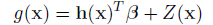
where h() is the trend of the model, is the vector of trend coefficients, and Z() is a stationary Gaussian process with zero mean that describes the departure of the model from its underlying trend. NESSUS assumes a constant trend function and is determined by least squares estimate. The covariance between outputs of Z() at points a and b is:

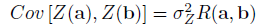
where R(), the correlation function is given by:

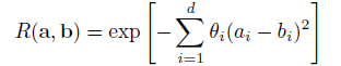
where d represents the number of design variables (dimensions), and is a scale parameter that governs the degree of correlation between the points in terms of dimension i. The expected mean and variance of the GP model prediction at point x are:

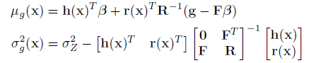
where r(x) is a vector containing correlations between x and each of the n training points, R is an n x n matrix containing the correlation between each pair of training points. g is the vector of response outputs at each of the training points, and F is an n x q matrix with rows h(x_i)^T (the trend basis function at training point i containing q terms; for a constant trend q = 1). This form of the variance accounts for the uncertainty in the trend coefficients , but assumes that the parameters governing the covariance function ( and ) have known values. The parameters and are determined through the maximum likelihood estimation. This involves taking a log of the probability of observing the response values g given the covariance parameters, given as:

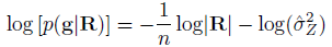
where |R| indicates the determinant of R, and is the optimal value of the variance given an estimate of . Maximizing the above equation gives the maximum likelihood estimate of which gives .

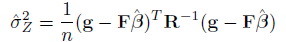
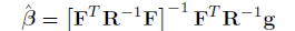
where is the generalized least squares estimate of from:

Thus everything is in place to get expected value and a predicted variance which gives a full Gaussian distribution. EGRA uses expected feasibility function to select the location at which a new training point should be added to the Gaussian Process model.

References:1. NESSUS Theoretical Manual, February 17, 2012, Section 9.1.1